





Transvalvular Pressure Gradient Modified Bernoulli Handheld Ultrasound
The modified Bernoulli equation turns a jet speed into a pressure gradient across a valve. A clinician reads the peak velocity of the jet on continuous wave Doppler. The equation multiplies the squared speed by four for the pressure the heart works against. A handheld carries the read to the bedside, where the gradient falls out of the trace in seconds.
What the gradient is
A pressure gradient is the difference in pressure across a valve. Blood flows from high pressure to low. A healthy valve lets it pass with almost no drop. A narrowed valve forces the blood through a small hole, which builds a large pressure difference across it. The heart must raise its pressure to drive the blood past the block. The gradient measures that extra work in millimetres of mercury. A large gradient marks a tight valve or a fast leak the heart strains against. A clinician grades a valve and follows it by the gradient over time. The number turns a vague murmur into a measured load. Each valve has its own normal gradient, near zero for an open valve. The gradient climbs with a tighter valve or a harder leak. A clinician takes the number as the pressure cost of the fault. The same number lets a clinician compare one visit with the last. A clinician quotes the gradient in millimetres of mercury.
The gradient is hard to measure directly inside the heart. A catheter can read the pressures on each side of the valve, an invasive step. Doppler reaches the same number from the speed of the jet alone. The jet speeds up exactly because the pressure drives it through the narrowing. A clinician takes that speed and works back to the pressure that caused it. The equation makes that step, from a velocity to a gradient, at the bedside. The handheld gives the gradient at the chair, in one read. A clinician once needed a catheter and a lab for the same number. The Doppler reads it from outside the chest in seconds. A clinician trades a procedure for a probe on the skin. The bedside number arrives in time to steer the visit. A clinician reads the gradient before the patient leaves the room. The number shapes the next step the same hour.
The Bernoulli principle behind it
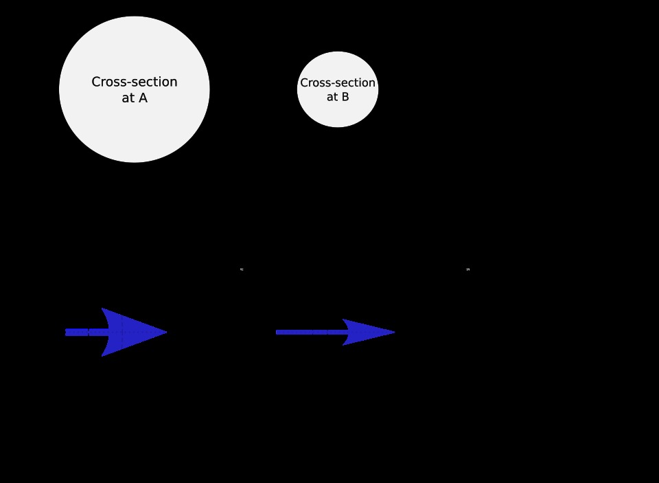
The equation rests on a law of flowing fluids. Energy in a smooth flow stays constant along its path. The energy sits in two pools: the pressure of the fluid and the motion of the fluid. A flow can trade one pool for the other along its path. A narrowing speeds the flow up, which draws energy from the pressure pool into the motion pool. The pressure falls by exactly the energy the speed gains. A clinician sees the principle in a river that quickens through a gorge. The same trade plays out when blood crosses a tight valve. The law carries the name of Daniel Bernoulli, who set it out for flowing fluids. The pressure and the speed move in opposite directions along a smooth flow. A clinician needs only the idea that speed gained means pressure lost. The valve speeds the blood, so the pressure across it must fall. A clinician holds that one idea behind every gradient read. The speed the Doppler reads is the pressure turned into motion.
A narrowing in a pipe shows the trade plainly. Blood in the wide channel runs slow under a high pressure. The same blood speeds up through the narrow throat. The faster the throat flow, the lower the pressure there. The drop across the narrowing is the gradient a clinician wants. A faster jet at the throat marks a larger drop across it. The valve is the narrowing. The fast throat jet is the leak or the stenotic flow. A clinician reads the throat speed off the Doppler and turns it into the drop. The wide channel before the valve holds a slow flow at a high pressure. The throat of the valve holds a fast jet at a low pressure. A clinician aims at the throat jet, since it carries the speed the equation needs. The drop across the throat is the gradient the heart works against.
The full law writes the pressure drop from three pieces. The first piece comes from the change in speed across the narrowing, the convective term. The second comes from the flow speeding up and slowing within the beat, the inertial term. The third comes from friction along the walls, the viscous term. Each piece adds to the pressure the flow loses across the valve. The three together give the exact drop a catheter would read. A clinician rarely needs all three for a clean valve jet. The convective term holds the change in speed across the valve. The inertial term holds the push needed to speed the flow up within the beat. The viscous term holds the rub of the blood on the walls. A clinician keeps the convective term for a sharp valve jet and lets the other two go. The convective term carries almost the whole drop across a clean valve. A clinician leans on it for the bedside read.
The heart simplifies the law in the common case. The inertial term fades for a steady jet read at its peak. The viscous term stays small across a short narrowing like a valve. The two small terms drop away. The convective term carries the gradient alone. A clinician keeps only the change in speed across the valve. The drop in the small terms is what lets a clinician read a gradient from speed alone. The equation shrinks to a single workable form. The inertial term counts only when the flow is still speeding up. A clinician marks the peak after the flow has settled, where that term has faded. The viscous term counts only across a long rough channel. A valve is short, so the rub of the blood on its walls stays small.
The convective term itself has a fixed shape. The pressure drop runs as half the fluid’s density times the change in the speed squared. Blood has a near-constant density across patients. A clinician folds that density and the unit conversion into one number. That number works out close to four for blood and the usual units. A clinician need not carry the density or the constant, only the four. The drop then reads as four times the squared speed, the form a clinician uses. The density of blood runs near 1.06 grams per millilitre in every patient. Half that density, turned into millimetres of mercury, lands close to four. A clinician trusts the four across patients for that reason. The constant changes only with a fluid the heart never pumps. The full constant works out near 3.97 for blood. A clinician rounds it to four with no loss at the bedside.
Reading the velocity for the gradient
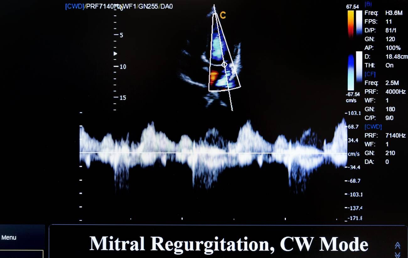
Continuous wave Doppler reads the speed the equation needs. A clinician finds the jet on colour and lays the beam down it. The mode reads the fastest blood on the line, which catches the peak of the jet. The trace draws a filled envelope. The peak sits at its outer edge. A clinician marks the peak and reads its speed in metres per second. The beam must run along the jet, since an off-axis beam reads the speed low. A small error in the speed grows fourfold in the gradient, so a clinician fills the envelope first. A clinician centres the jet in the colour box to aim the beam down its core. The mode reads along the whole line, so it finds the fastest blood wherever it sits. A clinician sweeps the probe and watches the peak rise to its tallest. A faint envelope reads the speed low and undercalls the gradient. A clinician angles the probe a few degrees at a time to chase the peak. The tallest clean envelope holds the true speed.
The peak velocity gives the peak gradient by the equation. A clinician squares the peak speed and multiplies by four. A traced envelope gives a mean gradient, averaged across the beat. The machine averages the gradient over the beat from that tracing. A clinician takes the peak for a quick number. The mean gives a steadier one. A clinician keeps the same units across visits to compare the numbers. Both come off the same trace in the one study. A clinician marks the peak with a tap once the trace is clean. The machine reads the gradient off the marked speed at once. A clinician checks the number against the look of the jet on colour. A clinician saves the peak velocity with the gradient for the record. The handheld stores the trace and the gradient with the study.
The simplified equation and its terms
The simplified equation is short: the gradient is four times the velocity squared. A clinician reads a velocity in metres per second and gets a gradient in millimetres of mercury. A jet at three metres a second gives a gradient near thirty-six. A jet at four gives sixty-four. The squared term means a small rise in speed lifts the gradient a long way. A clinician runs the squared speed in the head or reads it off the table. The table sets out the gradient for each velocity at a glance. A jet at two metres a second gives a gradient near sixteen. A jet at five gives a hundred. The gradient quadruples when the speed doubles, by the squared term. A clinician sees the steep climb straight from the table. A clinician runs a round velocity in the head for a quick gradient. A jet near three and a half metres a second lands close to fifty.
| Peak velocity | Pressure gradient (4V²) |
|---|---|
| 1 m/s | 4 mmHg |
| 2 m/s | 16 mmHg |
| 3 m/s | 36 mmHg |
| 4 m/s | 64 mmHg |
| 5 m/s | 100 mmHg |
| 6 m/s | 144 mmHg |
The equation drops one term a clinician should watch. The blood already moving before the valve carries a speed of its own. The full form subtracts that proximal speed: the gradient is four times the difference of the two squared speeds. A clinician ignores the proximal speed when it runs low, under about one metre a second. The simplified form then holds. The proximal speed matters when it runs high, in a tight outflow or a fast forward flow. A clinician adds the proximal speed back when it climbs, for an honest gradient. A proximal speed of one metre a second adds only four to the gradient, small enough to ignore. A proximal speed of two metres a second adds sixteen, large enough to subtract. A clinician weighs the proximal speed before dropping it. The ASE recommendations on aortic stenosis set out when each form applies.
The simplified equation gives a peak gradient from the peak velocity. A clinician marks it fast, straight off the tip of the trace. A traced envelope gives a mean gradient, averaged across the whole beat. The mean runs lower than the peak, since it counts the slower parts of the beat too. A clinician reports both for a fuller read of the valve. A clinician traces a clean beat for the mean and skips a noisy one. The two numbers frame the load from its top and its average. The Doppler peak gradient is the highest instant of the whole beat. A catheter quotes a peak-to-peak gradient between two separate pressure peaks. A clinician keeps the two numbers apart when comparing the methods. The mean gradient agrees best across the two. A clinician quotes the mean gradient when comparing reads across machines. The mean steadies a number a single peak might swing.
The equation reads a pressure gradient, leaving the valve area to other measures. A clinician reads the gradient for the pressure the heart fights. The flow rate sways the gradient: a weak pump drives a low gradient through even a tight valve. A clinician treats a low gradient with care, since a weak heart can hide a tight valve behind it. A clinician pairs the gradient with a flow-independent measure for the full grade. The valve area holds up when the flow runs low. A clinician reads the gradient and the area together for a grade that stands. A gradient and a valve area answer two halves of the question: the pressure load on the heart now, and the size of the opening whatever the flow. A clinician takes a severe area with a low gradient as a real tight valve under a weak pump. A clinician reads the dimensionless index when the area is hard to measure clean. The ratio grades the valve and skips the chamber width.
Where it goes wrong
The equation has limits a clinician must respect. A high speed before the valve breaks the simplified form, so a clinician then subtracts the proximal speed. A long tunnel-like narrowing adds friction the equation skips, which makes the read less exact. Pressure recovery trips the read in a small aorta or a prosthetic valve: the pressure climbs back downstream, so the Doppler reads a gradient higher than a catheter would. A clinician allows for that gap in those settings. The equation reads a flow-driven gradient, so a sluggish flow reads a low number despite a tight valve. A clinician checks the flow and the proximal speed before trusting the gradient. The number holds best on a clean jet with a normal flow ahead of it. The catheter settles a case the Doppler and the picture leave in doubt. A clinician notes any clash between the gradient and the rest of the study. The catheter reads the pressures direct when the doubt holds.
Across the valves
The same equation reads every valve in the heart. A stenotic aortic valve drives a fast forward jet. The gradient grades the narrowing. A leaking valve fires a backward jet. The gradient reads the pressure gap that drives the leak. A clinician reads each jet with the same four-times-squared rule. The jet changes from valve to valve. The equation behind it stays the same. A clinician reads an aortic jet from the apex and a mitral jet from the same window. The beam finds each jet on colour first. The four-times-squared rule turns each speed into its own gradient. A clinician learns the rule once and carries it across the valves. A clinician keeps the beam near zero to the jet, since an angle reads the speed short. The cosine of the angle scales the speed the mode reads.
The tricuspid jet turns the equation into a lung pressure. A clinician reads the leak’s speed, applies the four-times-squared rule, and adds the right atrial pressure for the pressure in the lungs. A prosthetic valve carries its own built-in gradient, read against the model’s normal range. A bileaflet mechanical valve recovers pressure that lifts its Doppler number above the true one. A clinician learns each prosthesis by the gradient its design runs. The chart sets what counts as a high gradient for that valve. The equation serves a shunt across a hole in the wall the same way. A clinician carries the one rule to every jet on the handheld. A clinician aims at the pulmonary valve jet for the gradient out to the lungs. The same rule reads a coarctation jet in the aorta. A clinician applies it to any fast flow a narrowing drives. The one equation covers the whole exam.
What the gradient guides
The gradient grades a valve and tracks it over time. A clinician takes a high gradient as a tight valve or a hard-driven leak. The number sets where a valve sits on the scale of severity. A clinician follows the gradient across visits to catch a valve on the move. A rising gradient warns of a narrowing that tightens. A clinician dates each gradient so the trend stands clear. The handheld reads the same number in the clinic itself. A clinician plots the gradient against the date to read the trend. A steady climb over the visits marks a valve that tightens for real. A single high reading can come from a fast heart or a thin patient. A clinician trusts a trend over one number. A clinician carries the trend in the device from visit to visit. A rising line over the years tells more than any one read.
The gradient guides the moment to act. A clinician refers a valve once the gradient and the symptoms cross the line for surgery. A severe gradient with symptoms sends a patient toward a new valve or a repair. The number times the referral before the heart gives way. A clinician weighs the gradient beside the chamber sizes and the function each visit. A clinician acts on a trend across visits more than a single reading. The bedside number starts that decision early. A clinician weighs the gradient with the symptoms and the chamber sizes. A high gradient alone rarely sends a patient to surgery. The whole picture, gradient and all, times the referral. A clinician reads the number as one strong voice in that call. A clinician brings the gradient to the heart team for the decision. The team weighs it with the imaging and the patient’s wishes.
The handheld puts the gradient in reach at every visit. A clinician finds the jet, marks the peak, and reads the gradient in under a minute. The pocket probe runs the same equation the cart machine runs. A clinician grades a valve at the chair, the ward, or the clinic. The number reaches a clinician from the trace alone. A clinician carries the whole gradient read in a coat pocket. The equation turns a speed a clinician can see into a pressure a clinician can act on. A clinician brings the same equation to the chair, the ward, and the clinic. The pocket probe needs no cart and no second machine. A clinician reads a gradient where a patient sits and acts on it the same hour. The one rule travels with the probe to every patient. A clinician saves the trace and the gradient to the record from the same screen. The number joins the patient’s chart in the one step.
Common questions about the Bernoulli gradient
How does the modified Bernoulli equation work?
The modified Bernoulli equation turns a jet speed into a pressure gradient. A clinician reads the peak velocity of the jet on continuous wave Doppler. The equation multiplies the squared speed by four for the gradient in millimetres of mercury. A jet at three metres a second gives a gradient near thirty-six.
What is the simplified Bernoulli equation for a valve gradient?
The simplified equation is the gradient equals four times the velocity squared. A clinician reads the velocity in metres per second from the Doppler trace. The four folds in the density of blood and the unit conversion. A clinician reads the gradient straight off the squared speed.
Why does the equation multiply by four?
The four comes from the physics of the flow and the units. The pressure drop runs as half the blood’s density times the change in the squared speed. The density of blood and the conversion to millimetres of mercury work out close to four. A clinician carries only the four and leaves the density and the constant in the background.
What is the difference between peak and mean gradient?
A clinician reads a peak gradient from the fastest moment of the jet, off the tip of the trace. A traced envelope gives a mean gradient, averaged across the whole beat. The mean runs lower than the peak, since it counts the slower parts too. A clinician reports both for a fuller read of the valve.
When does the modified Bernoulli equation fail?
The equation can mislead in a few settings. A high speed before the valve calls for the full form, with the proximal speed subtracted. A small aorta or a prosthetic valve recovers pressure downstream, so the Doppler reads a gradient higher than a catheter. A weak pump drives a low gradient through even a tight valve. A clinician checks the flow and the proximal speed before trusting the number.
About the Author
Julien Mercier
Senior R&D Engineer · Medical Ultrasound Transducer Development
Senior R&D Engineer with an M.S. in Applied Physics and over 15 years of experience in medical ultrasound transducer development, specializing in the design verification and performance testing of high-frequency imaging transducers. Currently leading the development and verification of the company’s next-generation high-frequency linear-array transducer, responsible for imaging performance evaluation and reliability analysis in preclinical testing. Brings extensive hands-on experience in piezoelectric element tuning, beamforming parameter optimization, and system-level performance testing.