


The DSP and SIMD Instructions on the Cortex-M4
The DSP instructions on the Cortex-M4 are an extension to the standard instruction set that runs fixed-point and integer signal math at high speed. A single-cycle multiply-accumulate, saturating arithmetic, and SIMD operations sit on the same core that runs the control code. These instructions turn the inner loop of a filter or a transform from a long routine into a few cycles. A design that runs signal processing in fixed point reaches for them to hold its work inside the time the loop allows.
What the DSP extension is
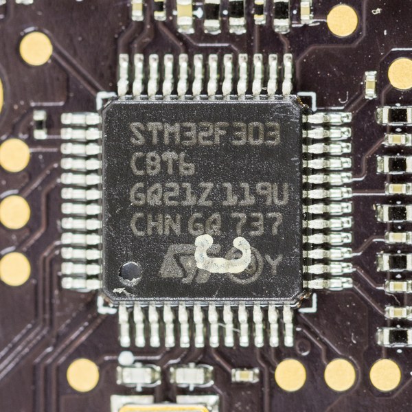
The Cortex-M4 carries a set of DSP instructions on top of the Thumb-2 instruction set the Cortex-M3 already runs. These instructions handle the integer and fixed-point math at the heart of signal processing: the multiply-accumulate, the saturating add, the packed SIMD operation. Arm documents them as running signal processing operations directly on the Cortex-M4, on the same core as the control code. The floating-point side of that work sits in a separate unit, the subject of its own guide. This extension is what makes a Cortex-M4 a capable fixed-point signal processor. The instructions belong to the Armv7E-M architecture, the base every Cortex-M4 implements, so a part marked as a Cortex-M4 carries them. They grew out of the digital signal processing world, where a multiply-accumulate that runs every cycle is the measure of a chip. Before the M4, a signal product paired a microcontroller with a dedicated DSP chip, two parts and two programs on one board. The extension folded those roles into a single part. The savings land in the bill of materials, the board area, and the firmware a team maintains. One interrupt, one clock domain, and one debug session now cover the whole job. That consolidation reads as the moment Arm brought signal processing into the mainstream microcontroller, on a part a motor or audio team already programs in C.
Inside the inner loop, the tight piece of code a filter or a transform runs over and over, the instructions earn their keep. A multiply-accumulate is the core step of that loop, and the DSP path runs it in one cycle with the operands held in registers across the passes. The same step on a core without the extension breaks into a multiply, a separate add, and the loads to feed them, run one after another. That fold of the multiply and the add is the whole story of the M4’s speed on signal code. Counting the multiply-accumulates and dividing by the clock gives a near-exact time for the inner work, the number a design budgets against the sample period. A worst-case branch costs a known handful of cycles, so the budget holds on the heaviest input. A control engineer trusts that bound on a motor that a missed deadline would damage.
The timing comes out exact. Every pass through the loop costs the same handful of cycles.
The instructions that do the work
The multiply-accumulate is the workhorse of the set. It multiplies two values and adds the result to a running total in one instruction. The finite impulse response filter is a sum of products, so its whole inner loop is a chain of multiply-accumulates. The DSP extension runs each one in a cycle. That cycle count sets the filter’s speed. Sixty-four taps become sixty-four multiply-accumulates per output sample. The per-cycle rate sets how many samples a second the core can process. The accumulator holds a wider result than the inputs, so a long chain of products keeps its low bits through the sum. A 16-bit by 16-bit multiply lands a 32-bit product. The accumulator runs wider still to hold the running total of many such products. The extra width is what keeps a long filter accurate, since the small contributions of distant taps survive in the low bits of the sum. A design reads the accumulator width on the datasheet against the dynamic range its filter needs. The wide accumulator on the Cortex-M4 covers the common audio and control filters without an intermediate rescale. An overly long or high-gain filter can still demand a rescale partway through, the step a careful fixed-point design plans at the points its analysis flags. The library routines handle that scaling in their tested forms, the reason a careful team reaches for a proven routine on a long filter. A profiler still has the final say on the cycle budget the chain spends on the target part. Coefficient storage rounds out the picture, since a long filter holds its taps in flash and streams them past the multiply-accumulate. Reading those coefficients from flash at the right rate keeps the unit busy, so a design lays the tables out for a clean sequential fetch. Memory bandwidth, not the math, becomes the limit on the longest filters, where the instruction can outrun the data feeding it.
SIMD packs several small values into one 32-bit register and works on all of them together. Two 16-bit samples, or four 8-bit ones, ride in a single register. One SIMD instruction adds, subtracts, or compares both pairs at once. The two 16-bit lanes are independent, so a left and a right audio channel move through the same instruction stream in lockstep. Sixteen bits hold the resolution a consumer audio path needs, the reason audio is the natural home for the 16-bit SIMD operations. Audio runs in 16-bit samples, so a stereo or a multichannel stream moves through a SIMD path at twice the rate of a one-at-a-time loop. The SIMD multiply-accumulate runs two 16-bit products and adds both to the accumulator in a single instruction, which is where a filter on packed data gains its speed. Image and sensor data in 8-bit form pack four to a register, so a pixel or a sample loop clears four values per instruction. The SIMD compare and select instructions handle the threshold and clip steps a signal pipeline runs between its filters. A team that lays out its buffers in the packed form the lanes expect gets the full benefit, since the data flows through the SIMD path with no rearranging.
Saturating arithmetic clamps a result at the maximum or minimum of its range. Plain integer addition wraps around when it overflows. The wrap turns a loud peak into a sudden burst of noise. The saturating add holds the value at the limit, the behaviour audio and control code need. It does the clamp in the same instruction as the math, at no extra cycle. One wrapped sample in an audio stream is an instant pop, the worst kind of artifact in a product a person listens to. Saturation keeps the worst case to a soft clip, the same way an analog circuit limits at its rail. The DSP set carries saturating versions of the add, the subtract, and the multiply-accumulate, so a whole signal chain runs clamped from end to end. Rounding modes ride alongside, so a fixed-point result rounds to nearest and holds the output free of the bias a plain truncation adds. These details are the difference between a textbook filter and one that holds its specification on a real signal.
A dual multiply runs two 16-bit multiplies and sums the products in one instruction. Complex arithmetic and the core of a fast Fourier transform lean on that pattern. The complex multiply is four real multiplies and two adds, the work this instruction collapses into a pair of steps. Packed load and store instructions move two or four small values at a time. A packed move keeps the SIMD lanes fed. The data comes in and out in the same packed form the SIMD instructions expect, so the loop spends no cycles unpacking and repacking. Together these instructions hold a fixed-point signal loop close to one result per cycle. The barrel shifter on the core runs alongside them, so a scaling shift folds into a math instruction at no cost. Bit-field and count-leading-zeros instructions round out the set for the block-floating and normalization steps a fixed-point chain runs between stages. Count-leading-zeros finds the headroom in a value in one instruction, the basis of a fast normalization. The combination of these helpers and the core multiply-accumulate is what lets a hand-tuned loop reach close to the theoretical rate of the hardware.
Fixed-point is where they live
The DSP instructions work on integers and fixed-point numbers, the format an integer-only design uses for real values. The Q15 or Q31 number holds a fraction in an integer, scaled by a known power of two, the depth of which the FPU guide weighs against floating point. On a Cortex-M4 the DSP extension runs that fixed-point math at full speed, so a design with no floating-point unit still carries a real signal chain. A Q15 value packs into the same 16-bit slot a SIMD lane holds, so the fixed-point format and the SIMD instructions fit each other by design. Integer hardware does the work of a signal processor here, on the numbers a microcontroller already handles fast. That is the whole point of the extension. Scaling by a power of two costs nothing, since a binary point moves with a shift the barrel shifter folds into the math. That free scaling is part of why fixed-point holds its speed on the M4, where every step stays in the integer pipeline the core runs fastest. The choice between fixed-point and floating-point is a design decision the FPU guide takes up in full, weighing the engineering of scaling against the silicon of a hardware unit. These instructions speed the fixed-point path. For a part with the floating-point unit, the CMSIS-DSP library wraps the same routines in floating-point forms. Fixed-point holds an edge in power and in worst-case timing, the traits a battery sensor or a hard real-time loop values. The signal work that runs on the DSP extension stays in integers from the input sample to the output, on hardware every Cortex-M4 carries.
What they accelerate
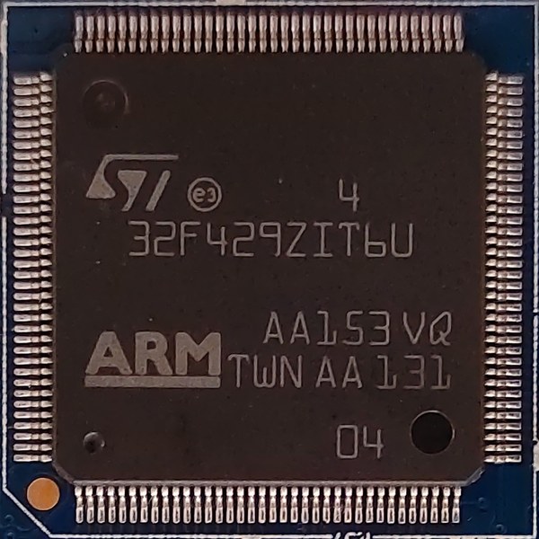
A finite impulse response filter is the first thing the DSP instructions speed. Its math is a sliding sum of products, a tap count of multiply-accumulates per output sample. The DSP extension runs that sum at one tap per cycle. The SIMD path doubles it again on 16-bit data, so a hundred-tap filter runs in real time on the same core. The filter length sets the cost, since each extra tap adds one multiply-accumulate per sample. Long filters that sharpen a band edge or reject a tone stay inside the budget on the DSP path at a sample rate a plain integer core could not hold.
An infinite impulse response filter, built as a chain of biquads, runs the same multiply-accumulate pattern with feedback. Each biquad is a handful of multiplies and adds per sample. The DSP extension and its saturating math run a stack of biquads inside an audio sample period. An equalizer, a crossover, or a tone control sits here. A biquad holds five coefficients and a little state, so a parametric equalizer with several bands stacks a handful of them in sequence. The DSP path runs the whole stack on every sample. A graphic equalizer or a speaker correction filter stays inside the audio budget that way. State storage matters as much as the math here, since each biquad keeps a small history a careful design holds at full precision. Truncating that state too early colours the sound, so a tuned filter keeps the extra bits the wide accumulator offers. The feedback in an IIR filter makes the saturating math matter, since a value that overflows in the feedback path can send the filter into oscillation. The saturating add holds the state inside its range. The filter stays stable through a loud transient.
The fast Fourier transform is the other heavy load. Its butterflies are complex multiply-accumulates, the exact pattern the dual-multiply instruction runs. A fixed-point FFT on the DSP extension turns a spectrum analysis from a slow batch job into a per-frame step. A vibration monitor, a power meter, or a software radio front end runs that transform in its loop. The dual-multiply instruction matches the complex butterfly at the heart of the FFT, so each stage moves through the data at the rate the hardware allows. A 256-point or 1024-point transform that once needed a separate chip now runs on the microcontroller between samples. The CMSIS-DSP FFT functions handle the bit-reversal and the twiddle factors, so a team gets a working transform from a single call. Real input and complex input forms cover the common cases, from a vibration spectrum to a modulation analysis. The inverse transform runs the same hardware in reverse for a design that synthesizes a waveform. A windowing step, a magnitude calculation, and a peak search all draw on the same DSP instructions around the transform itself. The magnitude step squares and sums the real and imaginary parts, two multiply-accumulates per bin, the kind of work the extension runs at full rate. A spectrum that updates several times a second on a microcontroller is the everyday result of these instructions working together. Window functions shape the input before the transform, a multiply of each sample by a stored coefficient, more multiply-accumulate work the extension runs at rate. Picking the FFT length trades frequency resolution against the cycles per frame, a budget a design sets against its update rate. Longer transforms resolve finer tones and spend more work per frame, so a vibration tool sizes its FFT to the fault frequencies it has to separate. A condition-monitoring sensor watches the spectrum of a bearing or a fan for the signature of a fault, all on the part that also reads the sensor and talks to the network. The transform, the magnitude, and the threshold check fit between the samples, the whole analysis on one Cortex-M4 in the field.
The CMSIS-DSP library puts these instructions to work with no hand-written assembly. It ships ready FIR, IIR, FFT, and matrix routines, each tuned to the DSP extension and the SIMD path. A team calls a function and gets the speed the instructions allow. The library covers fixed-point and floating-point forms, so the same call moves with the design from one core to another. The routines are tested and documented. They take the numerical risk out of a hand-coded filter. The schedule that would lose weeks to writing and verifying assembly instead drops in a library call and moves on.
Real products lean on these instructions every day. A motor controller runs its current-shaping filters in fixed point. A hearing aid runs its noise reduction inside a tiny power budget. A sensor node runs an FFT to classify a vibration. A wireless earbud runs its codec and its active noise cancellation in the same chip. Each one holds its signal math on a Cortex-M4. The cycle count stays a small fraction of what a plain integer core spends on the same work. The integration is the gain as much as the speed, since the signal work and the control work share one part, one toolchain, and one program. A wearable that reads a heart-rate sensor, filters the signal, and drives a display does all three on one Cortex-M4. The signal stage and the user-interface stage trade data in memory, with no inter-chip link to design or debug. The power story improves on the same path, since one active part draws less than two. A duty-cycled product runs its filter on a wake, posts the result, and sleeps, the whole cycle on a single low-power core.
Which parts have them, and using them
The DSP extension rides on the Cortex-M4, the Cortex-M7, and the Cortex-M33. Any part on one of those cores runs the instructions. Below them, the Cortex-M0, M0+, and M3 run the same signal math in plain integer code, several instructions per step. A design that leans on fixed-point signal work reads the core first, since the extension is what holds that work in real time. Above the M4, the Cortex-M55 and M85 carry Helium, a wider vector engine that extends the same idea for machine learning and heavier signal loads. For the bulk of audio, motor, and sensor work, the Cortex-M4 DSP extension is the rung a design settles on. A Cortex-M7 runs the same DSP instructions on a faster, dual-issue core for a heavier load. The instruction set carries across, so code written for the M4 moves up to the M7 with a recompile and gains the headroom. The decision for a new design reads the signal load against the clock the part offers. A filter and transform budget that fits an M4 at its clock stays on the M4. A load that overruns it moves to a faster M4 part or up to an M7. Those instructions are the constant across that range, the reason a team’s signal code keeps its value across a growing product line. Code density helps the cause, since the dense Thumb-2 encoding the M4 shares with the M3 packs the signal loop into less flash. A tight loop that fits the instruction prefetch runs without a stall, the last piece of the speed the hardware promises.
Using the extension takes little extra effort. The compiler emits the instructions when the build targets a Cortex-M4, so plain C with the right flag picks them up. The CMSIS-DSP library wraps the common routines, ready for a team to call. Intrinsics give direct access to a specific instruction where a hand-tuned loop needs it. The build flag for the core also turns on the right code path in the CMSIS-DSP library, so a single setting points the whole project at the M4 instructions. A team that starts from a CMSIS-DSP example reaches a working filter on day one and tunes from there. The library also documents the cycle cost of each routine, so a design budgets its signal chain before a line of custom code is written. A profiler confirms the number on the target part, the final check that the chain fits the loop. The payoff is signal processing at microcontroller cost. The same Cortex-M4 that runs the control logic runs the filters and transforms in fixed point, on one chip, in one program. A design names the heaviest signal math its loop runs. If that math fits the loop time on the DSP extension, the core does the whole job. These instructions are what let a plain microcontroller carry a load that once took a dedicated DSP chip.
| Instruction group | What it does | Signal work it speeds |
|---|---|---|
| Multiply-accumulate | multiply two values, add to a running total, in one cycle | FIR and IIR filter taps, dot products |
| SIMD add / subtract | two 16-bit or four 8-bit values handled together | audio streams, image and sensor data |
| Dual 16-bit multiply | two products summed in one instruction | complex math, FFT butterflies |
| Saturating arithmetic | hold a result at the range limit on overflow | audio peaks, fixed-point safety |
| Packed load / store | move two or four small values at once | feeding the SIMD lanes |
What is the difference between the DSP instructions and the FPU on a Cortex-M4?
The DSP instructions run integer and fixed-point signal math, such as a single-cycle multiply-accumulate and SIMD operations. The floating-point unit runs real-number math in hardware, the subject of its own guide. A Cortex-M4 part can carry the DSP extension, the FPU, or both, so a design checks the part for what it needs.
Do I need to write assembly to use the DSP instructions?
No. The compiler emits the instructions from plain C when the build targets a Cortex-M4. The CMSIS-DSP library wraps the common filters and transforms in ready functions. Intrinsics give direct access to a single instruction for a hand-tuned inner loop.
What does SIMD do for signal processing?
SIMD packs two 16-bit or four 8-bit values into one register and operates on them together. Audio and sensor data run in 16-bit samples, so a SIMD path processes a stereo or multichannel stream at twice the rate of a one-value-at-a-time loop. It doubles the throughput of a filter on packed data.
Can a Cortex-M0 or M3 run the same DSP code?
The math runs, in plain integer instructions, several per step. The Cortex-M0, M0+, and M3 lack the DSP extension, so a filter or transform takes more cycles there. A design that runs heavy fixed-point signal work in a fast loop reads the Cortex-M4 or higher for the extension.
Which DSP instruction is the workhorse?
The multiply-accumulate carries the bulk of signal work. It multiplies two values and adds the result to a running total in one cycle, the core step of every FIR and IIR filter and every dot product. The whole inner loop of a filter is a chain of these, so its single-cycle speed sets the filter’s rate.