Marcus Chen January 17, 2026

What is Battery SOC SOH Monitoring

Lithium-ion batteries lie. The voltage at the terminals tells a story contaminated by temperature, by current, by the electrochemical history of the past few hours. Extracting truth from this contaminated signal is what SOC SOH monitoring does.

SOC

SOC means state of charge. Ratio of remaining capacity to total capacity. Simple enough on paper.

But Q_max is a fiction. A 100 Ah cell fresh from the factory delivers 100 Ah at C/3 discharge, 25°C, between 4.2V and 2.5V. That same cell three years later delivers 82 Ah under identical conditions. Which number goes in the denominator? The original 100 Ah? The current 82 Ah? The answer determines whether a half-discharged old battery shows 41% SOC or 50% SOC. Neither is wrong. Both are defensible. No standard exists.

This definitional chaos explains why EV owners compare range displays and get confused. A Tesla at 50% and a Rivian at 50% represent different things depending on what each manufacturer decided Q_max means. Some use nameplate capacity and let SOC=0% creep upward as the battery ages. Others recalibrate periodically and keep SOC=0% anchored to the actual empty point. The choice is arbitrary, and almost nobody documents which convention they use.

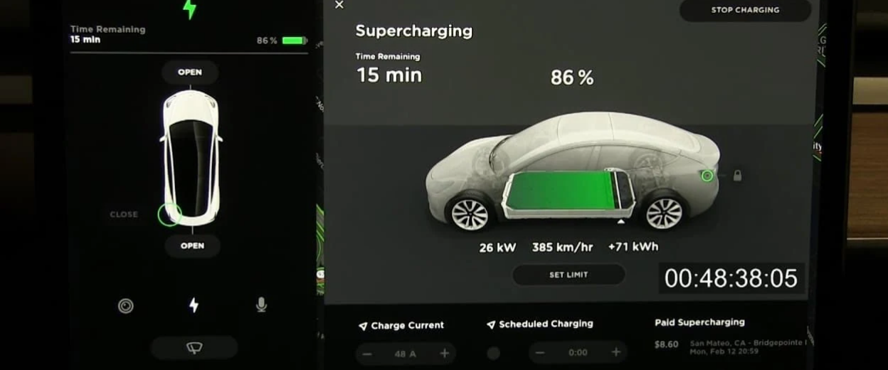
EV dashboard displays showing SOC percentages — numbers that mean different things across different manufacturers

The physical reality underneath SOC is lithium concentration in electrode particles. When fully charged, the graphite anode holds lithium in the form of LiC6. During discharge, lithium deintercalates from the anode, travels through the electrolyte, and intercalates into the cathode. SOC tracks this migration. But tracking it electrically means measuring voltage and current, neither of which directly reports lithium concentration.

SOH

State of health compresses years of electrochemical degradation into one number. The compression loses almost everything interesting.

Two degradation mechanisms dominate lithium-ion aging. Loss of lithium inventory (LLI) happens when lithium gets trapped in the SEI layer or plated as metallic lithium that cannot be recovered. Loss of active material (LAM) happens when electrode particles crack, detach, or undergo structural transformations that render them electrochemically inactive. LLI and LAM produce different symptoms. LLI shifts the voltage curve without changing its shape much. LAM changes the shape. A cell with 85% SOH from LLI behaves differently than a cell with 85% SOH from LAM. The single SOH number erases this distinction.

Battery aging is multidimensional — a single SOH percentage cannot capture the complexity of degradation mechanisms

The 80% threshold for end of life emerged from early EV programs where 80% capacity retention kept driving range above the threshold of customer complaints. Nothing electrochemical happens at 80%. Cells continue degrading smoothly through 75%, 70%, 65%. The threshold is marketing, not physics. Second-life applications exploit this gap, buying "dead" EV batteries and running them for another decade in stationary storage where reduced capacity and power matter less.

Resistance-based SOH tracks a different degradation axis. Internal resistance rises as contact resistances increase, as the SEI layer thickens, as electrolyte decomposition products accumulate. A cell with excellent capacity retention can have terrible resistance growth if the dominant degradation mode is electrolyte decomposition. The reverse also occurs. A single SOH number cannot capture both axes.

Coulomb Counting Works Until It Doesn't

The most straightforward SOC tracking method integrates current over time.

Measure current. Multiply by time. Accumulate. Done. Computational cost is negligible. Works on any microcontroller. No battery model required.

The problem is error accumulation. Current sensors have offset voltages that create phantom currents. A Hall sensor with 0.5% offset on a 200A system injects 1A of fake current. Over 24 hours, that 1A integrates to 24 Ah of error. For a 100 Ah battery, SOC drifts 24% per day without recalibration.

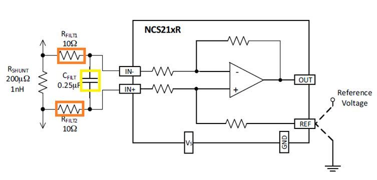
Precision current sensing — where millivolt-level errors accumulate into significant SOC drift over time

Temperature makes it worse. Hall sensor offset drifts with temperature. So does shunt resistor resistance. A shunt spec'd at 200 μΩ might be 210 μΩ at 80°C and 195 μΩ at -10°C. The current measurement error rides along with these drifts, accumulating into SOC error that only gets corrected when something else resets the estimate.

The "something else" is usually OCV calibration. Wait for the battery to rest, measure the open circuit voltage, look up SOC from a table, and reset the Coulomb counter to that value. But resting long enough for OCV calibration takes hours at low temperatures. A vehicle that runs all day without long parking periods accumulates drift with no reset opportunity. Some fleet operators see 10-15% SOC error by evening on vehicles that started the morning calibrated.

OCV Calibration

The open circuit voltage carries thermodynamic information about lithium concentration. In principle, OCV is a function of SOC alone (at fixed temperature). Measure OCV, look up SOC, done.

Reality is messier. After current stops, voltage relaxes toward equilibrium over timescales ranging from minutes to hours depending on temperature and SOC. The relaxation has multiple time constants corresponding to different physical processes: charge transfer kinetics decay in seconds, concentration gradients in the electrolyte decay in minutes, solid-state diffusion in particles takes hours. At -20°C, even the fast processes slow down. A battery parked overnight in winter may not reach true OCV by morning.

Cold weather dramatically extends voltage relaxation times — overnight parking may not be enough for true OCV equilibration

LFP chemistry amplifies the problem. The lithium iron phosphate cathode undergoes a two-phase reaction that produces a flat voltage plateau spanning 60% of the SOC range. Within this plateau, OCV changes by 15 mV over 50% SOC change. Voltage measurement uncertainty of ±3 mV corresponds to ±10% SOC uncertainty in the plateau region. NMC chemistry avoids this specific problem because its OCV curve has more slope, but LFP dominates in buses, commercial vehicles, and stationary storage. Engineers who design for NMC and then deploy on LFP learn this lesson expensively.

Hysteresis creates another trap. OCV measured after charging differs from OCV measured after discharging at the same SOC by 10-50 mV depending on chemistry. This is not a relaxation effect; it persists indefinitely and reflects path-dependent lithium ordering inside particles. An algorithm that ignores hysteresis and uses a single OCV-SOC lookup table will show SOC jumping when the battery switches from charging to discharging or vice versa.

Kalman Filters

The Extended Kalman Filter appears in almost every academic paper on SOC estimation. The appeal is obvious: a mathematically principled framework for fusing model predictions with measurements, automatically tracking uncertainty, handling noise optimally under Gaussian assumptions.

The battery model underlying most EKF implementations is an equivalent circuit: an OCV source, a series resistance R0, and one or two RC networks representing polarization dynamics. State vector is typically [SOC, V_c1, V_c2] where V_c1 and V_c2 are voltages across the RC elements. The observation equation relates terminal voltage to these states:

The EKF propagates this model forward and corrects using voltage measurements. The correction strength scales with dOCV/dSOC, the slope of the OCV curve. Where the slope is large (NMC across most of its range), voltage measurements strongly inform SOC. Where the slope is small (LFP plateau, overcharge and overdischarge regions of any chemistry), voltage provides almost no information and the filter runs open-loop.

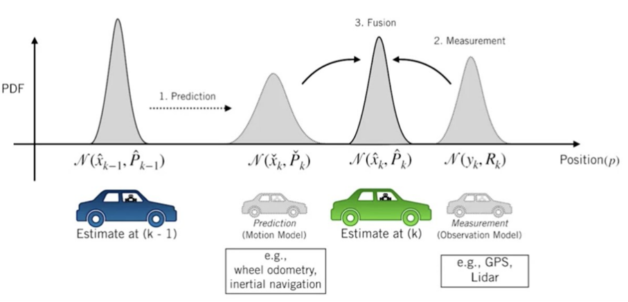
Kalman filtering fuses noisy measurements with model predictions — the mathematical elegance that dominates production BMS implementations

This is where EKF implementations diverge between academic and production quality. Academic papers report RMSE on datasets collected at 25°C with carefully controlled current profiles. Production systems operate from -30°C to +55°C with current profiles determined by driver behavior and road conditions. The model parameters R0, R1, C1, R2, C2 all vary with temperature, SOC, current magnitude, current direction, and aging state. An EKF using fixed parameters works brilliantly in the lab and fails in the field.

Production systems use lookup tables mapping parameters to operating conditions. The tables require extensive characterization: pulse tests at every combination of temperature and SOC, repeated on fresh cells and aged cells, across cell-to-cell variation within production lots. Populating these tables costs months of continuous testing and consumes expensive test channel time. Skipping this characterization and using nominal datasheet values produces systematic SOC error that no amount of algorithmic sophistication can fix.

The noise covariance matrices Q and R require tuning that no textbook explains adequately. Q represents model uncertainty. R represents measurement uncertainty. R can be estimated from sensor datasheets. Q has no physical basis; it must be tuned empirically by running the filter on representative data and adjusting until tracking behavior satisfies some subjective criterion. Different engineers tuning the same filter arrive at different Q values. The resulting filters behave differently. Published papers rarely report Q tuning procedures, making results difficult to reproduce.

UKF, PF, and Diminishing Returns

The Unscented Kalman Filter replaces EKF's linearization with sigma-point sampling, capturing nonlinearity more accurately. The improvement matters where OCV(SOC) is highly nonlinear: LFP plateau edges, extreme SOC regions. For NMC in the 10-90% SOC range, UKF and EKF produce nearly identical results. The 3× computational overhead buys nothing.

Particle filters promise even better handling of nonlinearity and non-Gaussian distributions. In simulation studies, particle filters outperform Kalman variants. In production, nobody uses them. The computational cost scales with particle count, typically 100-1000× more expensive than EKF. The improvement in SOC accuracy does not justify this cost when model parameter uncertainty dominates algorithm limitations.

Neural Networks

LSTM networks achieve 0.5-1.5% RMSE on benchmark datasets. Transformers push this below 0.5%. The papers are impressive. The deployment stories are scarce.

Training data requirements exceed what most organizations can produce. A network learning to estimate SOC must see examples covering the full operating space: temperatures from -30°C to +55°C, SOC from 0% to 100%, currents from trickle charge to fast discharge, aging states from fresh to end-of-life. Factorial combinations explode quickly. Sampling this space densely enough for reliable learning requires months of continuous testing on dozens of cells.

Neural networks achieve impressive benchmark results — but the gap between academic papers and production deployment remains vast

Field data offers volume without labels. Real vehicles generate terabytes of voltage, current, and temperature data. But the true SOC is unknown. Supervised learning requires labels. The circular dependency between needing SOC estimates to train SOC estimators creates a bootstrapping problem with no clean solution.

Generalization fails catastrophically across cell manufacturers. A network trained on LG cells produces garbage on Samsung cells even when both use the same chemistry and similar specifications. Manufacturing variations in electrode coating thickness, electrolyte formulation, formation protocols produce voltage signatures that differ enough to confuse networks. Transfer learning helps but requires labeled data from the target domain, which recreates the original data problem at smaller scale.

Deployment on BMS hardware faces memory and compute constraints that academic implementations ignore. A modest LSTM consuming 200 KB of parameters and requiring 300,000 multiply-accumulates per inference exceeds the budget of cost-optimized automotive MCUs. Quantization to 8-bit integers helps but adds 0.2-0.5% SOC error from precision loss. Model distillation can shrink networks 5-10× but adds development time and complexity.

The interpretation problem makes safety certification difficult. When a neural network outputs wrong SOC, no amount of inspection reveals why. The weights are inscrutable. Functional safety standards require demonstrating correct behavior under all foreseeable conditions. For neural networks, this requires exhaustive testing that approaches the cost of generating training data. Model-based methods offer easier certification paths because failure modes trace to identifiable parameter errors.

SOH Estimation Operates on Different Timescales

SOC estimation must run in real-time, updating every 10-100 milliseconds. SOH estimation operates on timescales of days to months. This separation permits methods impractical for SOC.

The gold standard remains full capacity measurement: charge fully, discharge fully at a standardized rate, integrate current. Accuracy reaches ±0.5% under controlled laboratory conditions. Field application is limited because vehicles cannot be taken out of service for multi-hour tests. Partial discharge methods estimate capacity from segments of normal operation but propagate SOC endpoint errors into capacity estimates.

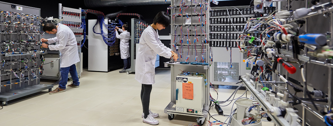
Battery testing laboratory — where months of characterization produce the lookup tables that production systems depend on

Incremental capacity analysis differentiates charge throughput with respect to voltage: IC = dQ/dV. The resulting curve shows peaks at voltages where phase transitions occur in electrode materials. Peak positions shift with lithium loss; peak heights decrease with active material loss; peak widths increase with resistance growth. Tracking these features over time enables diagnosing which degradation mechanisms are active.

The signal processing burden is heavy. Numerical differentiation amplifies noise. Measurement noise of 10 mV produces derivative noise proportional to 10 mV divided by voltage step, which typically exceeds signal amplitude in flat curve regions. Heavy filtering is mandatory before peak detection, and the filter parameters affect peak positions enough to corrupt trend analysis if not carefully controlled.

Electrochemical impedance spectroscopy provides richer degradation information by measuring complex impedance across frequencies from 10 mHz to 10 kHz. The Nyquist plot reveals distinct features: ohmic resistance from the high-frequency intercept, SEI layer impedance from the first semicircle, charge transfer impedance from the second semicircle, diffusion limitations from the low-frequency tail. Tracking these features over life enables diagnosing specific degradation mechanisms rather than just aggregate capacity loss.

EIS requires specialized equipment and 15-30 minutes per measurement. Embedded implementations exist but demand analog hardware precision exceeding typical BMS designs. The technique remains confined to laboratory characterization and specialty applications where detailed degradation information justifies cost.

Hardware Determines the Ceiling

Algorithm accuracy cannot exceed measurement accuracy. A BMS with ±5 mV voltage error and ±2% current error will never achieve ±1% SOC accuracy regardless of algorithm sophistication.

Analog front end ICs dominate voltage measurement. The best automotive-grade parts achieve ±1-2 mV total error across temperature, including ADC nonlinearity, reference drift, and multiplexer leakage. Less expensive parts reach ±5-10 mV. For NMC chemistry where OCV changes 300 mV over the full SOC range, ±2 mV corresponds to ±0.7% SOC resolution. For LFP in the plateau region where OCV changes 15 mV over 50% SOC, the same ±2 mV error corresponds to ±7% SOC resolution.

Battery Management System electronics — where millivolt precision determines the ultimate accuracy ceiling

Current sensing splits between shunts and Hall sensors. Precision shunts achieve 0.1% accuracy but require amplifying millivolt signals in the presence of hundreds of volts common mode. The amplifier offset voltage, typically 25-150 μV, translates to 0.1-0.6 A offset through a 250 μΩ shunt. Offset drift over temperature accumulates into SOC error during extended operation.

Hall sensors provide galvanic isolation but sacrifice accuracy. Open-loop Halls achieve 1-3% accuracy with significant temperature dependence. Closed-loop Halls reach 0.2-1% at higher cost. Fluxgate sensors deliver 0.01-0.1% accuracy for applications where cost is secondary to precision.

Temperature measurement affects SOC estimation through parameter lookup. Model parameters vary 2-5× between 0°C and 40°C. A temperature error of ±5°C causes parameter lookup errors that propagate into model mismatch. NTC thermistors provide ±0.5-2°C accuracy at low cost. Placement matters as much as accuracy: a thermistor on the BMS board measures board temperature, which can differ from cell temperature by 10°C during high-rate operation.

Production Reality

The distance between academic papers and production code is measured in years and millions of dollars.

Algorithm development starts in MATLAB or Python with floating-point arithmetic and unlimited memory. Porting to embedded C with fixed-point arithmetic and 32 KB RAM introduces precision losses, execution time constraints, and numerical stability problems that do not appear in the comfortable development environment.

The journey from algorithm to production — where 90% of effort goes to validation, certification, and manufacturing processes

Hardware-in-the-loop testing validates timing and fault handling. Functional safety certification demands diagnostic coverage metrics that require extensive fault injection testing. Documentation for certification often exceeds the code it describes.

Vehicle integration exposes interactions invisible in isolation: EMI from motor inverters corrupting communication, thermal gradients causing parameter mismatches, vibration causing intermittent connector faults. Field data from production fleets reveals problems affecting 0.1% of vehicles that never appeared in pre-production testing.

The calendar time from algorithm concept to production release spans 2-4 years for automotive. The algorithm represents perhaps 10% of total effort. The remaining 90% goes to validation, certification, documentation, and manufacturing process establishment.